
Unsupervised Classification
An illustration with 2D synthetic data
OK. Let us first play with a very simple 2D data set created by us by sampling from two identical normal (=Gaussian) distributions with centres displaced.
library("mvtnorm")
set.seed(10)
setA <- rmvnorm(1000,c(0,0),matrix(c(1,0,0,1),2,2))
setB <- rmvnorm(1000,c(3,3),matrix(c(1,0,0,1),2,2))
mock.data <- rbind(setA,setB)
plot(mock.data)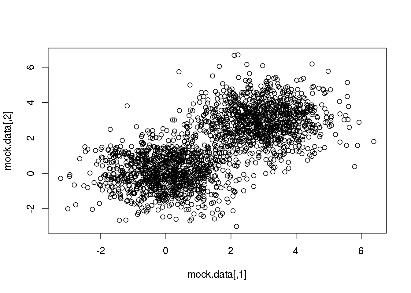
The Expectation-Maximization algorithm
We start by randomly selecting two points that we will take as starting solution.
rc <- sample(1:dim(mock.data)[1],2)
plot(mock.data)
points(mock.data[rc,],pch=16,col="seagreen",cex=2)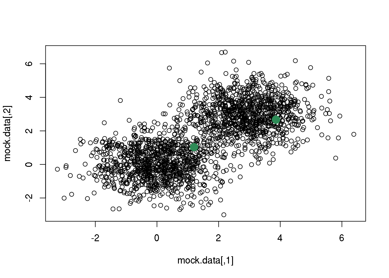
We will then take this two points as the centres of the two clusters. We could have tried three or more clusters.
If these two points are the centres of the two clusters, each cluster will be made up of the points that are closer to each centre. Closer is a word that implies many things. In particular, it implies a distance and a metric. In the following, I will assume that the metric is Euclidean, but you have various choices (Euclidean, Manhattan, L\(\infty\)) that you should consider before applying (most) clustering algorithms.
A quote from Elements of Statistical Learning
“An appropriate dissimilarity measure is far more important in obtaining success with clustering than choice of clustering algorithm. This aspect of the problem … depends on domain specific knowledge and is less amenable to general research.”
If you decide to use the euclidean distance, take into account is definition:
\(d(x,y) <- sqrt(\sum_i^n (x_i-y_i)^2)\)
If dimension \(i\) has a range between 0 and, say, \(10^6\) while dimension \(j\) only goes from 0 to 1, differences in \(i\) will dominate the distance even if they only reflect noise.
Also, the choice of metric dictates the position of the centres, as we shall see later.
Now, we define a function to compute 2D distances:
d <- function(center,data){
  s1 <- t(apply(data,1,"-",center))
  s2 <- s1^2
  s3 <- apply(s2,1,sum)
  d <- sqrt(s3)
  return(d)
}
… and will assign each point to the closest centre (in the euclidean sense)
# We define a function to do that
E <- function(data,centres){
  # First some definitions...
  n.data <- dim(data)[1]
  n.dims <- dim(data)[2]
  n.cl <- dim(centres)[1]
  dists <- matrix(NA,n.data,n.cl)
  # Then, compute distances from each point to each cluster centre
  for (i in 1:n.cl) dists[,i] <- d(centres[i,],data)
  # ... and define the cluster as the index with the minimum distance
  cluster <- apply(dists,1,which.min)
  return(cluster)
  }

centres <- mock.data[rc,]
# Call the function
cluster <- E(mock.data,centres)

plot(mock.data,pch=16,col=cluster)
points(mock.data[rc,],pch=16,col="seagreen",cex=2)
We see that this assignment produces a linear boundary defined by the points at the same distance from the two centres. But it does not look right. This is because we have only taken the first step of \(k\)-means.
The second step consists of recalculating the positions of the cluster centres given the cluster assignments (partition) above:
# We define a function to recalculate the centres...
M <- function(data,cluster){
  labels <- unique(cluster)
  n.cl <- length(labels)
  n.dims <- dim(data)[2]
  means <- matrix(NA,n.cl,n.dims)
  for (i in 1:n.cl)  means[i,] <- apply(data[cluster==labels[i],],2,mean)
  return(means)
}

means <- M(mock.data,cluster)

plot(mock.data,pch=16,col=cluster)
points(mock.data[rc,],pch=16,col="seagreen",cex=2)
points(means,pch=16,col="green",cex=2)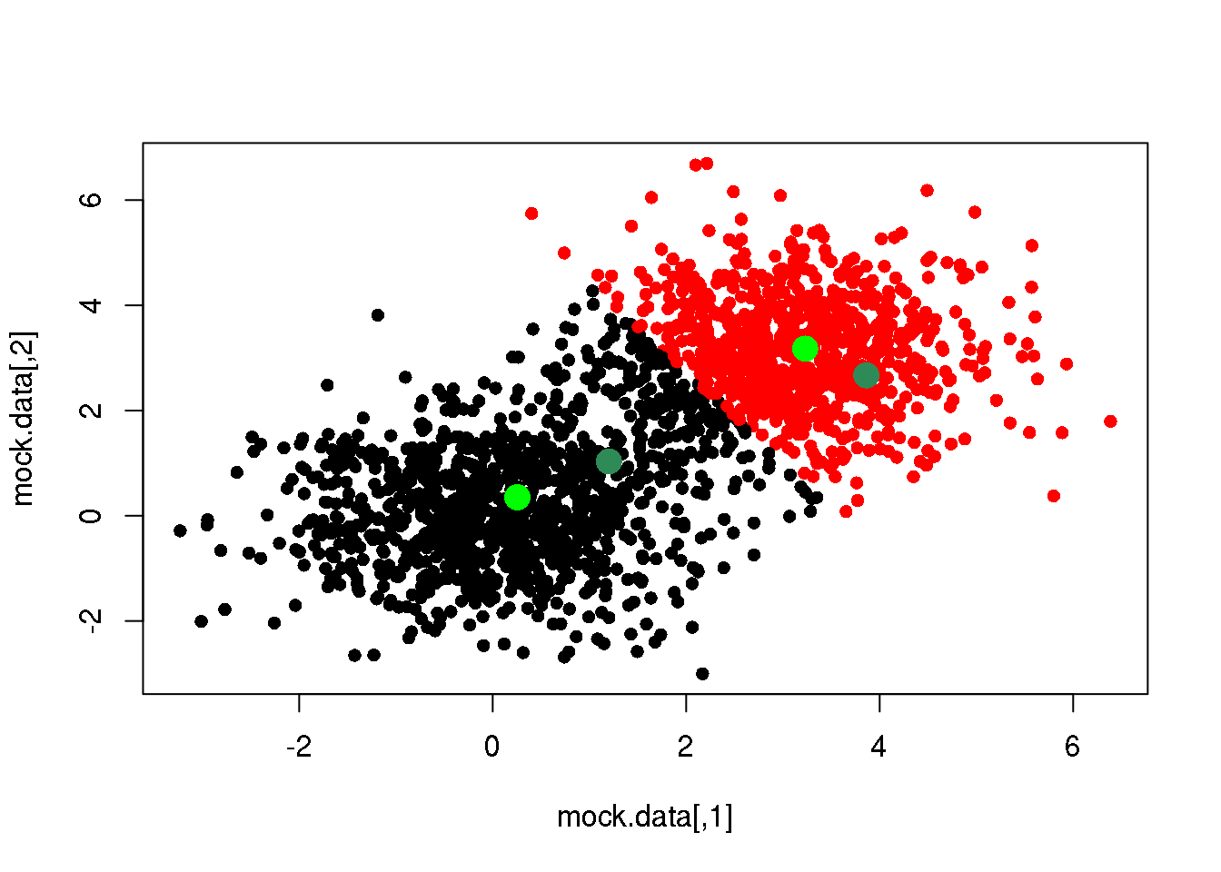
So far, we have taken several decisions: 1. we have chosen to measure (dis-)similarity between elements using the euclidean distance; 2. we decided to attach a label (cluster) depending to the minimum distance to the centres; 3. and finally, we have decided to recalculate the cluster centres as the mean of (and only of) the points with a given cluster label (we could have used the median, or the closest point to the mean or the median, or…)
Now, let us redo the cycle (steps 1 and 2) one more time:
cluster <- E(mock.data,means)
plot(mock.data,pch=16,col=cluster)
points(means,pch=16,col="seagreen",cex=2)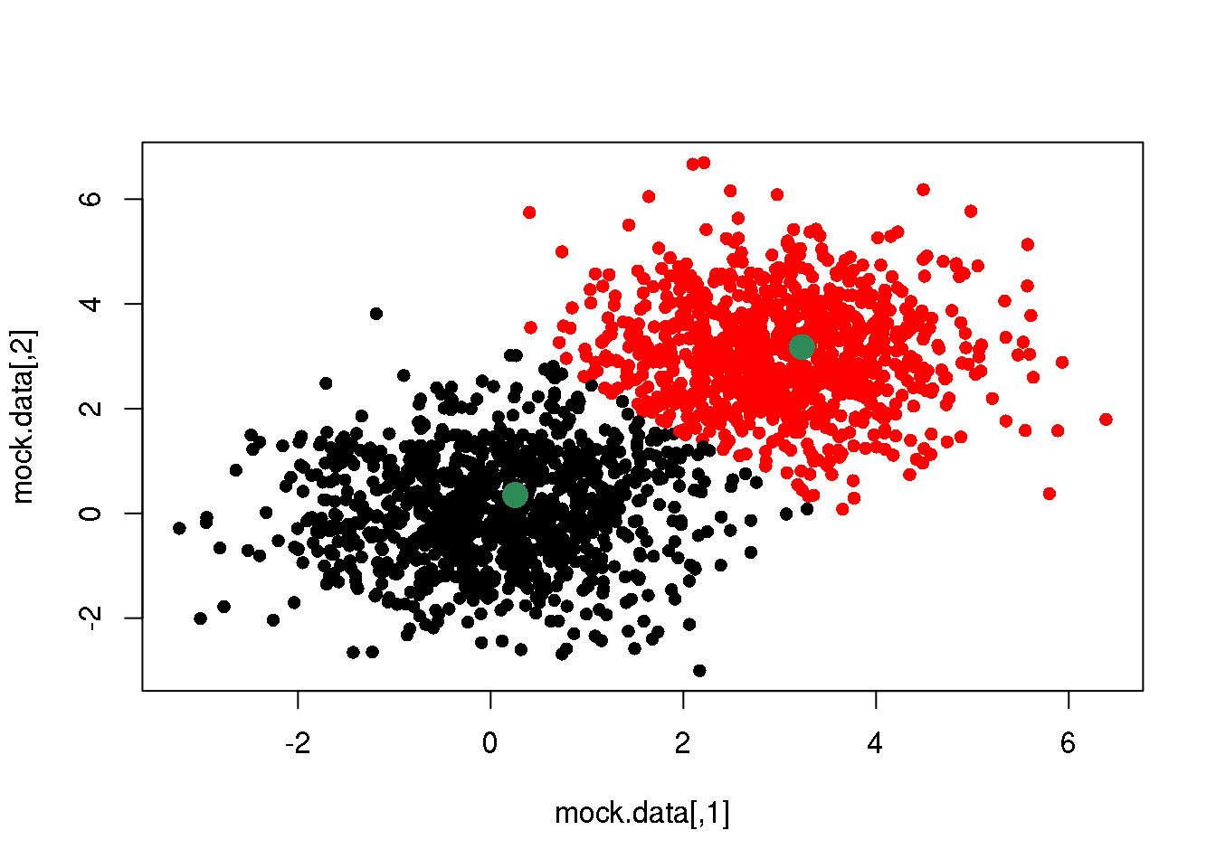
OK. If we do this over and over again, until one cycle does not produce any change in the cluster assignments and means, we have done a \(k\)-means clustering.
km <- kmeans(mock.data,2)
plot(mock.data,col=km$cluster,pch=16)
points(km$centers,pch=16,col="seagreen",cex=2)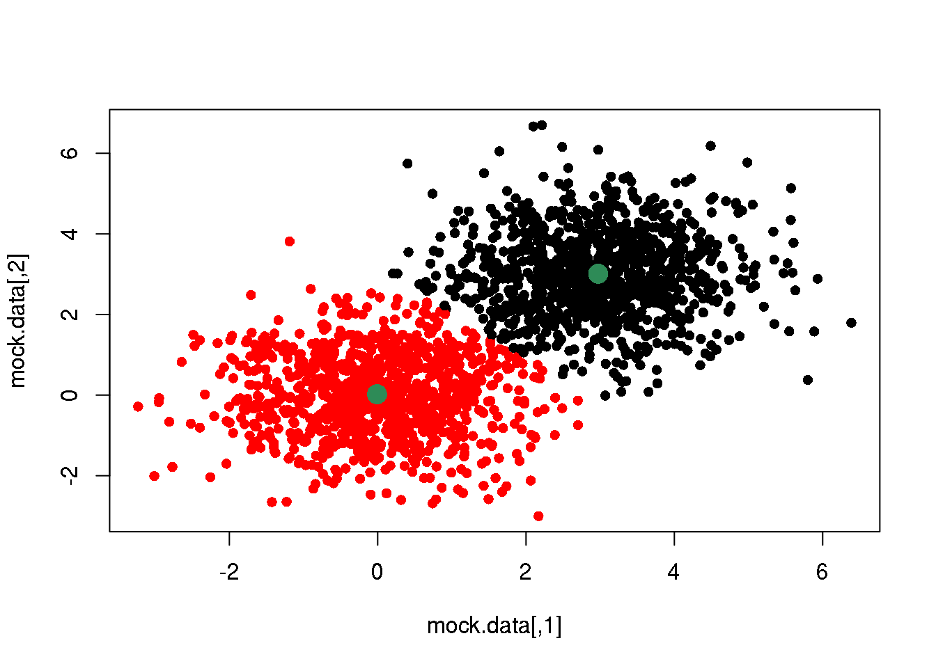
The OGLE data set
So far, so good…
But life is not 2D, and if Science only dealt with 2D problems, most of the field of multivariate statistics would be pointless.
Let us have a look at a real (yet still simple) data set:
data <- read.table("OGLE.dat",sep=",",header=T)
attach(data)

plot(logP,WI,pch=".")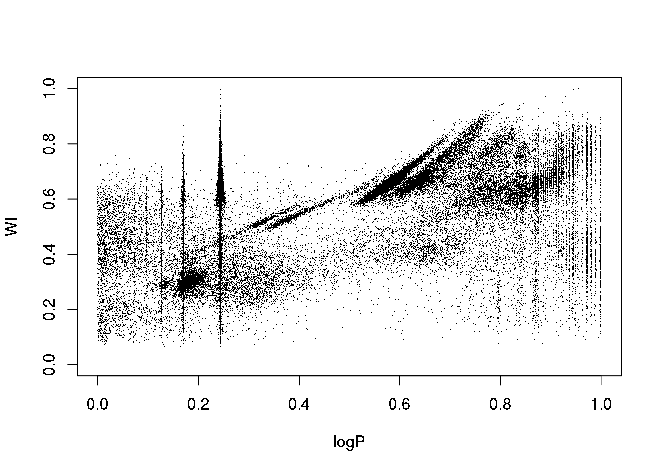
The data set corresponds to the OGLE III survey of periodic variable stars in the Large Magellanic Cloud, and the plot above shows only two of the 5 attributes that describe each source: 1. the logarithm of the period of each cycle 2. the logarithm of the first Fourier term amplitude 3. the ratio of amplitudes of the first two Fourier terms 4. the phase difference between the first two Fourier terms 5. the V-I colour index 6. the (reddening free) Wessenheit index
The 5 attributes have been re-scaled between 0 and 1.
The educated eye sees the classical pulsators, some extrinsic variability, and spurious structure.
Unfortunately, the spurious structure overlaps with true variability (like, for example, \(\gamma\) Doradus stars and Slowly Pulsating B-type variables that can have periods around 1 day). Therefore, careless cleaning (as the one practitioned below) is just wrong.
The variability zoo is beyond the scope of this lectures, so you will have to have faith and believe me.
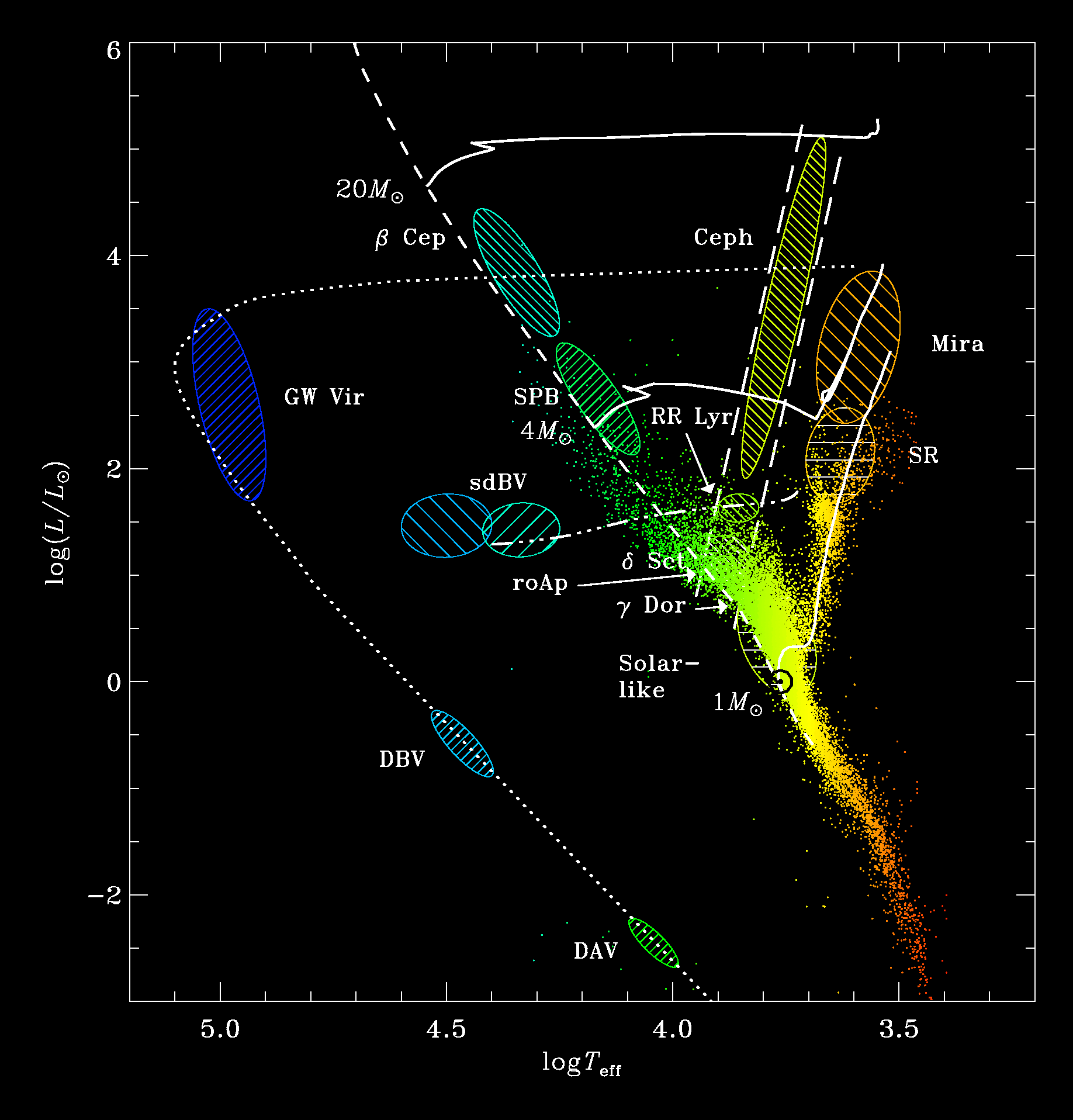
Just as a teaser, I cannot help show you the HR diagram:
OK. Let us do a quick and dirty cleaning just so that you can play with the data…
mask <- (logP < 1-0.754 & logP > 1-0.76) | (logP < 1-0.827 & logP > 1-0.833) | (logP < 1-0.872 & logP > 1-0.873)
data <- data[!mask,]
attach(data)
plot(logP,WI,pch=".")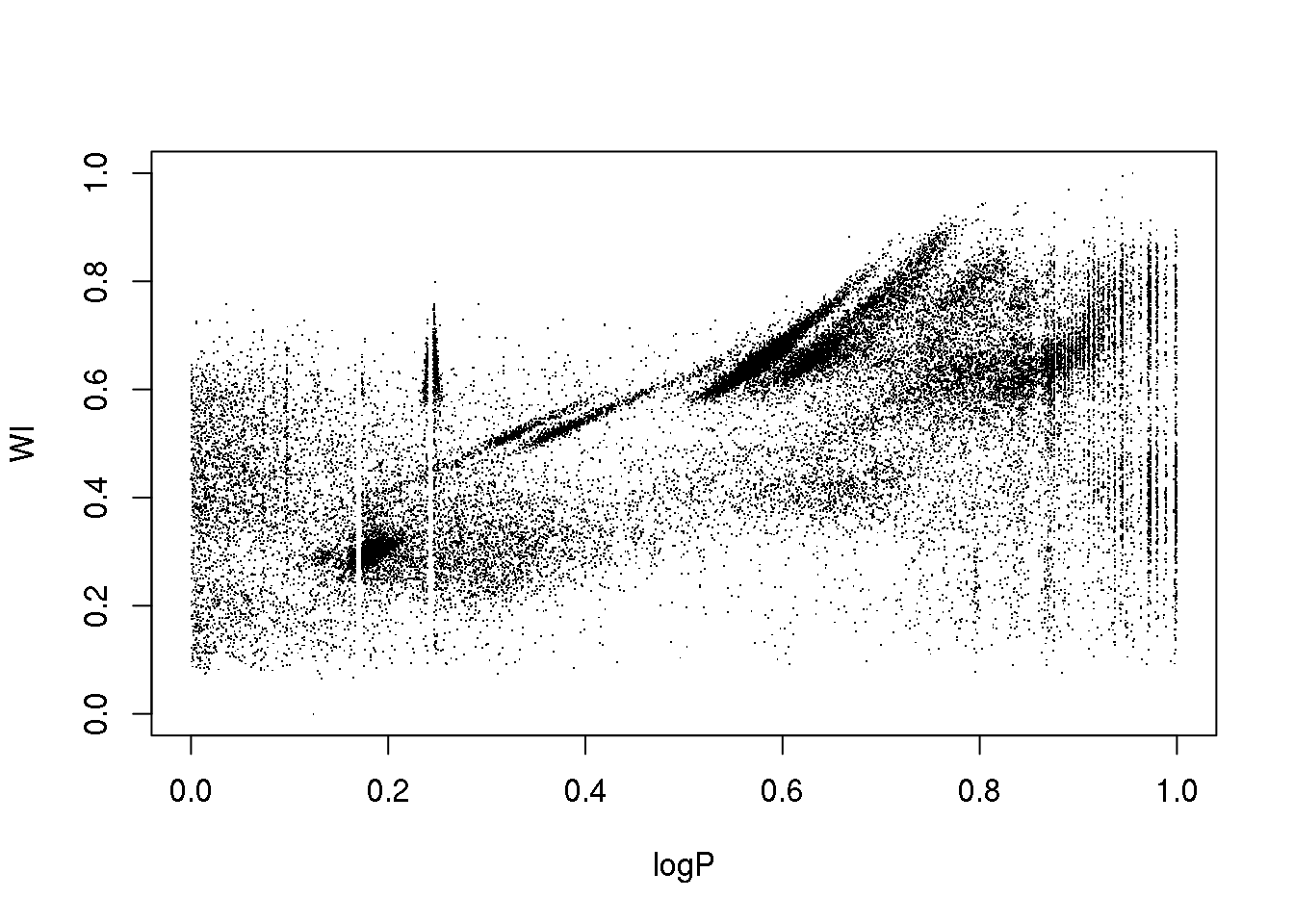
Now, let us try to apply \(k\)-means to the OGLE data set. How many clusters will we try to derive? So far, I have given you no heuristic to decide on the optimal number of clusters. So let us try 10, just for fun:
km10.ogle <- kmeans(data,10)
plot(logP,WI,pch=".",col=km10.ogle$cluster)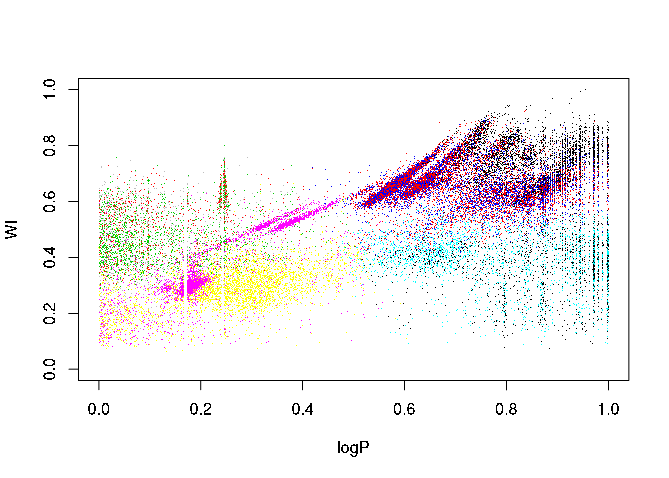
This is certainly too few. Let us try with 25 clusters:
set.seed(5)
km25.ogle <- kmeans(data,25,iter.max = 20)
plot(logP,WI,pch=".",col=km25.ogle$cluster)
points(km25.ogle$centers[,c(1,6)],col=seq(1,25),pch=16,cex=2)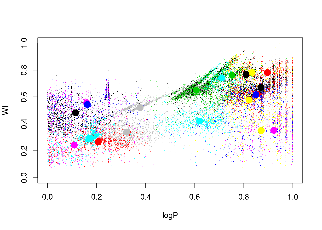
OK: we see that eclipsing binaries are separated from the RR Lyrae stars. But the Lpng Period Variables sequences are mixed up, despite their being clearly separated in this 2D projection.
Let us try a different random seed, just to check that this was not a poor initialization:
set.seed(15)
km25.ogle <- kmeans(data,25,iter.max=20)
plot(logP,WI,pch=".",col=km25.ogle$cluster)
points(km25.ogle$centers[,c(1,6)],col=seq(1,25),pch=16,cex=2)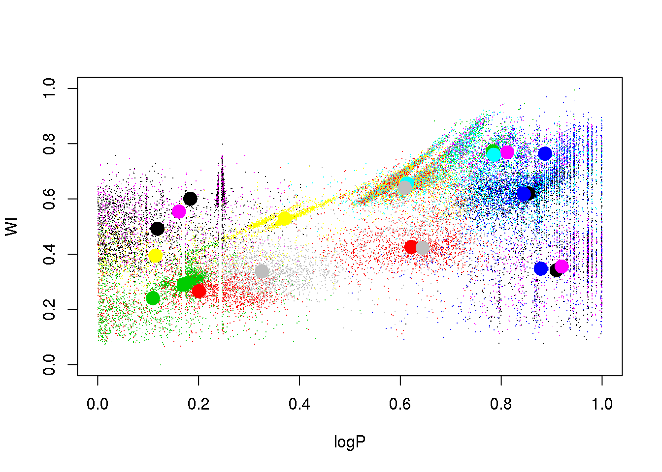
Ooooops. The LPVs are still mixed, and the RR Lyrae got mixed up now with the eclipsing binaries.
The problem is the inclusion of an attribute that is only useful for a subset of classes:
plot(logP,phi21,pch=".",col=km25.ogle$cluster)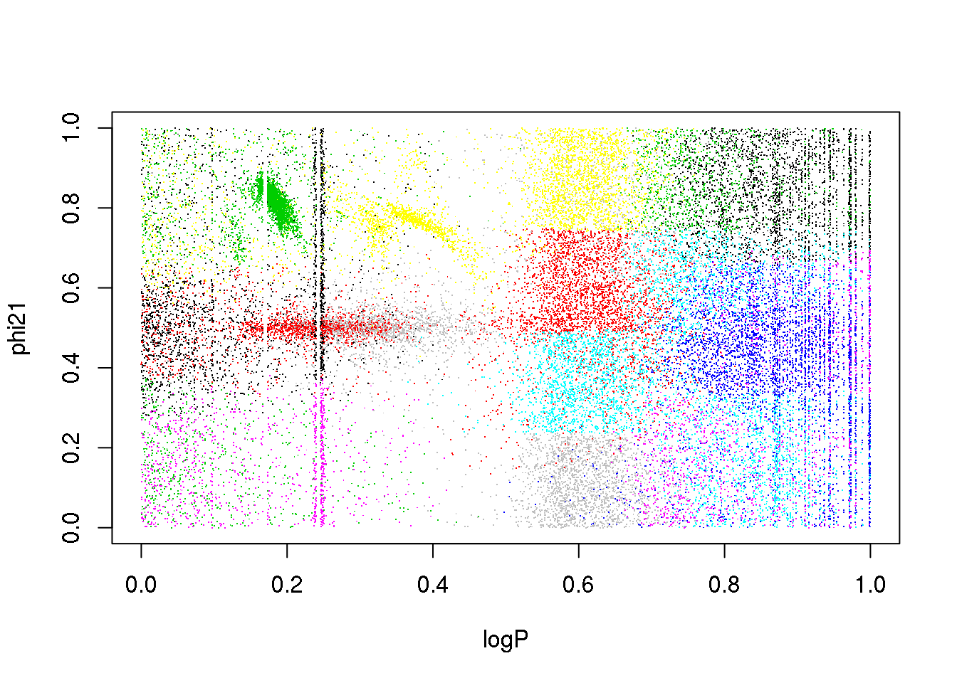
What happens if I remove it?
set.seed(15)
km25.ogle <- kmeans(data[,-4],25,iter.max=20)
plot(logP,WI,pch=".",col=km25.ogle$cluster)
points(km25.ogle$centers[,c(1,5)],col=seq(1,25),pch=16,cex=2)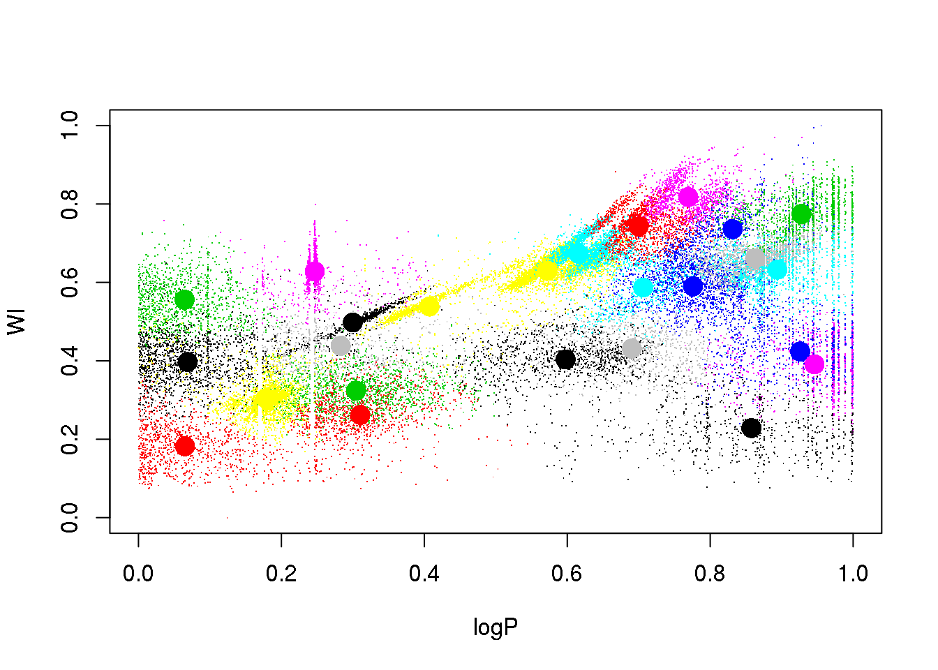
A bit better, but still insatisfactory. One would wish to remove the dependency on the random initialization, and have a guide as to how many clusters there actually are in the data. More on this later…
Expectation-Maximization
OK. \(k\)-means is just an algorithm that represents a special case of a more general one known as Expectation-Maximization.
I will show you what it is by working out a practical example (learn by doing).
First, let me generate again a synthetic data set taylor to highlight the main advantage of going from the particular (\(k\)-means) to the general:
set.seed(10)
setA <- rmvnorm(1000,c(0,0),matrix(c(3,0,0,3),2,2))
setB <- rmvnorm(1000,c(3,3),matrix(c(1,0.99,0.99,1),2,2))
setC <- rmvnorm(1000,c(-1,4),matrix(c(1,-0.9,-0.9,1),2,2))
mock.data <- rbind(setA,setB,setC)
plot(mock.data)
So this is our data set. It is two-dimensional to help illustrate the underlying concepts and the maths, but we could perfectly well try in more than 2D.
Our data set consists of 3000 points drawn from three normal (=Gaussian) distributions with varying shapes and orientations. The key point to keep in mind is that the three distributions overlap in 2D space.
Let us see the performance of our now-known \(k\)-means technique.
km <- kmeans(mock.data,3)
plot(mock.data,col=km$cluster,pch=16,cex=.5)
points(km$centers,pch=15,col="orange")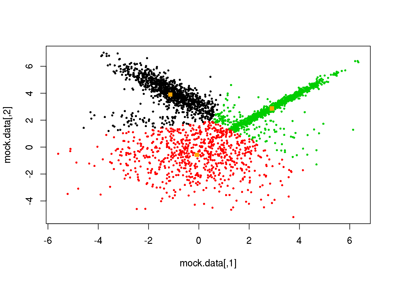
Not bad, but it clearly can be improved. We see that the distance threshold is a reasonable approach, but returns clusters of roughly the same area (not true for more than three clusters). Hence the inappropriate cluster assignments.
Let me now propose a different algorithm based on the concepts introduced yesterday by René. Remember that René introduced the concept of generative model for supervised learning. It naturally lead him to define the probability of the data given the model parameters, the so-called likelihood.
Since we know the true model underlying our data set, let us write down a log-likelihood function that would tell us what model parameters maximize the probability of our data set given the model.
\[\mathcal{N}(\vec{x})=\frac{1}{(2\pi)^{k/2}}\frac{1}{\Sigma^{1/2}}\cdot e^{-\frac{1}{2}((\vec{x}-\vec{\mu})^T\Sigma^{-1}(\vec{x}-\vec{\mu}))}\]
loglikNormal <- function(D,means,Sigmas,cluster){
  labels <- unique(clusters)
  n.cl <- length(labels)
  loglik <- 0
  for (i in 1:n.cl)
  {
  logliki <- apply(means[i,],1,dmvnorm,x=D[cluster==i,],sigma=Sigma[,,i])
  logliki <- apply(logliki,2,sum)
  loglik <- loglik+logliki
  }
  return(loglik)
}
It has for parameters: the data, the means and covariance matrices of the normal distributions, and… the cluster assignements! For three clusters and 3000 points, we have 6+9+3000. And this is 2D only.
The space of parameters is HUGE: the means, the covariance matrices, and partitions! It is impossible that we test all possible combinations these 3015 parameters. How could we conceivably compute the likelihood in this high-dimensional space?
Solution 1: the EM algorithm
(Solution 2 is… go Bayesian and use MCMC!)
Let us simplify the problem: assume that the three normals have the same (unknown) covariance, that the covariance is diagonal and that the two variances are equal.
Then, you have \(k\)-means! Except for a few subtleties…
Now, let us remove some constraints: the covariance matrices can be arbitrary, and we try to maximize the log-likelihood. Difficult eh? Then, let us use the EM algorithm.
The EM algorithm is an iterative algorithm to find (local) maxima of the likelihood function or the posterior distribution for models with a large amount of latent variables. It alternates the following two steps: * the E(xpectation) step: given a set of model parameters, it computes the expected value of the latent variables. And… * the M(aximization) step: given the latent values, computes the model parameters that maximize the likelihood.
rc <- sample(1:dim(mock.data)[1],3)
plot(mock.data,pch=16,cex=.5)
points(mock.data[rc,],pch=16,col="seagreen",cex=2)

# We start with a random selection of points as centres...
means <- mock.data[rc,]
Sigmas <- array(0,dim=c(2,2,3))
# And diagonal (unit) matrices for the covariances.
Sigmas[1,1,]=1
Sigmas[2,2,]=1

# And here is the function to compute the expected values of the
# latent variables:
E <- function(data,means,Sigmas)
{
  n.cl <- dim(means)[1]
  probs <- matrix(NA,nrow=dim(data)[1],ncol=n.cl)
    for (i in 1:n.cl)
  {
  probs[,i] <- dmvnorm(x=data,mean=means[i,],sigma=Sigmas[,,i])

  }
  cluster <- max.col(probs)

  return(cluster)
}

# OK. let us do it:
cluster <- E(mock.data,means,Sigmas)

points(mock.data,pch=16,cex=.5,col=cluster)
points(mock.data[rc,],pch=16,col="seagreen",cex=2)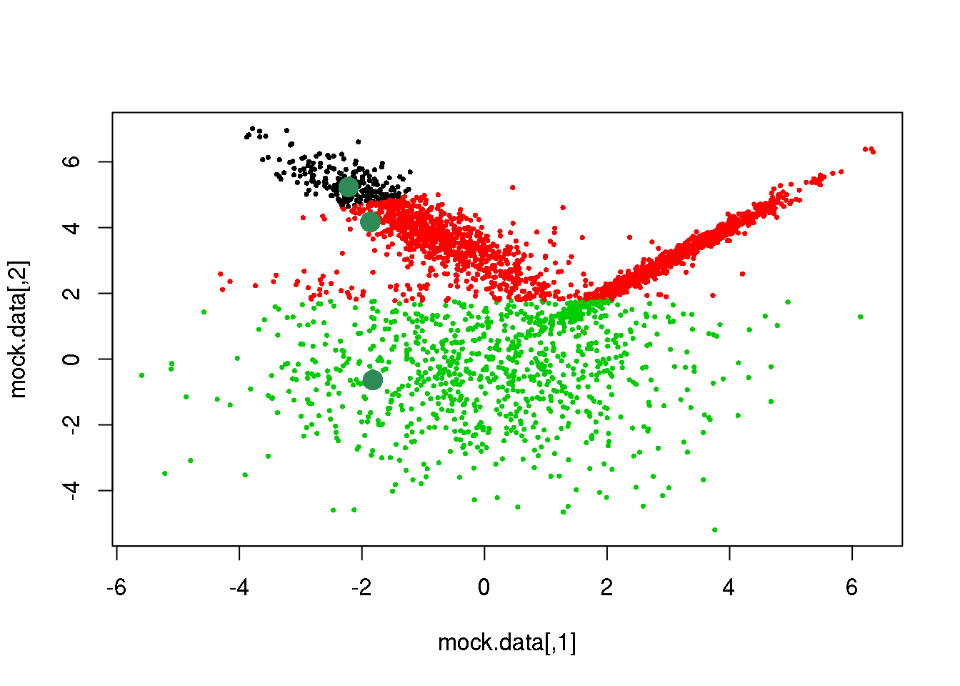
We have accomplished the E-step, let us now complete the first cycle:
M <- function(data,cluster){
  n.cl <- length(unique(cluster))
    for (i in 1:n.cl)
  {
      means[i,] <- apply(data[cluster==i,],2,mean)
      Sigmas[,,i] <- cov(data[cluster==i,])
  }
  M <- list(means=means,covariances=Sigmas)
  return(M)

}

plot(mock.data,pch=16,cex=.5)
points(mock.data[rc,],pch=16,col="seagreen",cex=2)
points(mock.data,pch=16,cex=.5,col=cluster)
points(mock.data[rc,],pch=16,col="seagreen",cex=2)

parameters <- M(mock.data,cluster)
points(parameters$means,pch=16,col="orange",cex=2)
cluster <- E(mock.data,parameters$means,parameters$covariances)
plot(mock.data,pch=16,cex=.5,col=cluster)
points(parameters$means,pch=16,col="orange",cex=2)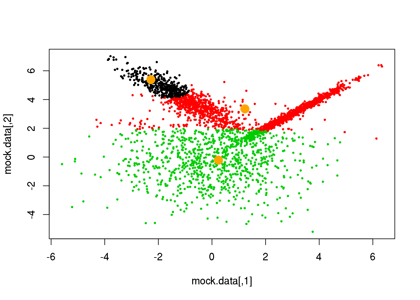
Looks fine! Now, let us do it until a cycle results in no changes in either the model parameters or the cluster assignments:
for (i in 1:50)
{

parameters <- M(mock.data,cluster)
cluster.new <- E(mock.data,parameters$means,parameters$covariances)
ndiff <- sum(cluster!=cluster.new)
print(ndiff)
cluster <- cluster.new
plot(mock.data,pch=16,cex=.5,col=cluster)
points(parameters$means,pch=16,col="orange",cex=2)
if(ndiff==0) break
}
## [1] 221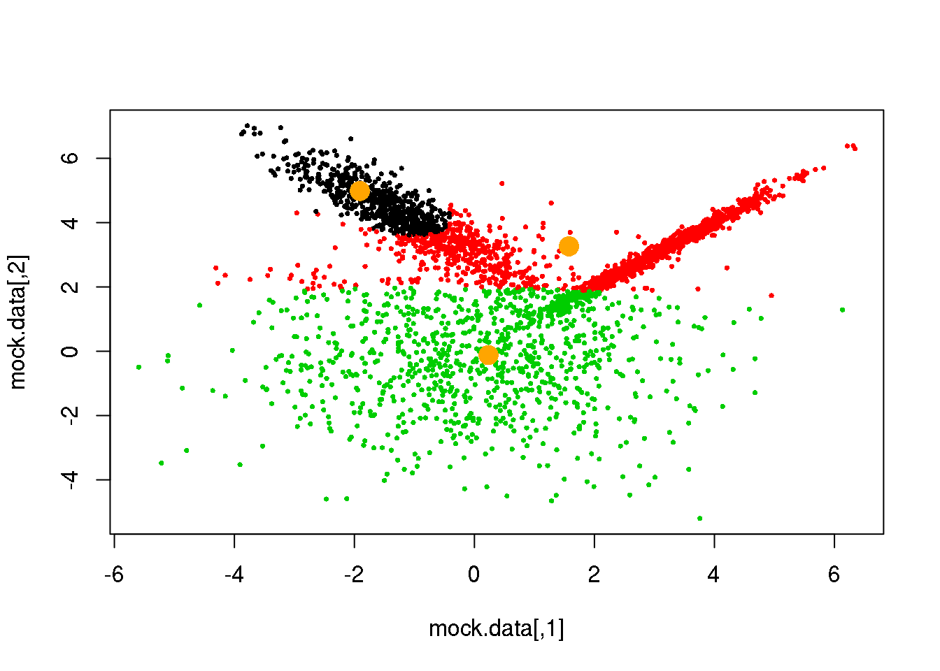
## [1] 204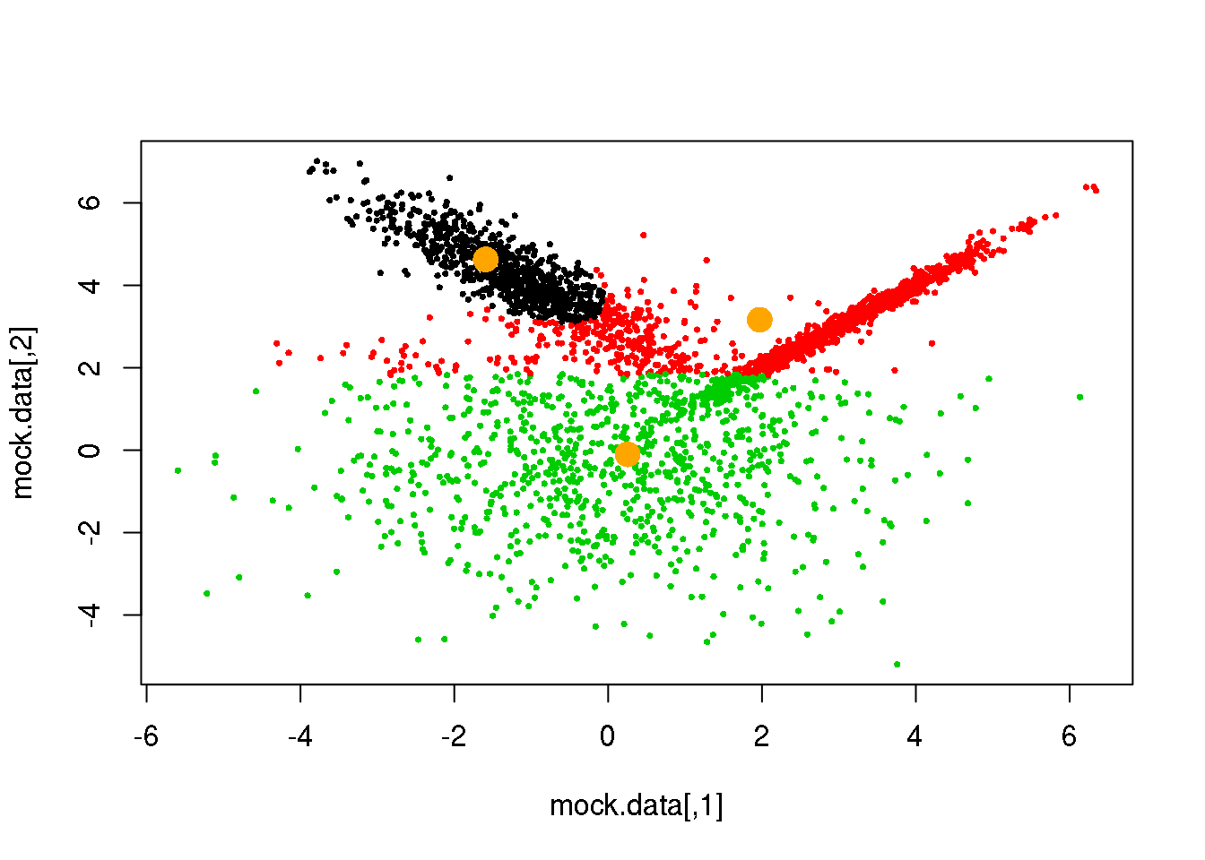
## [1] 189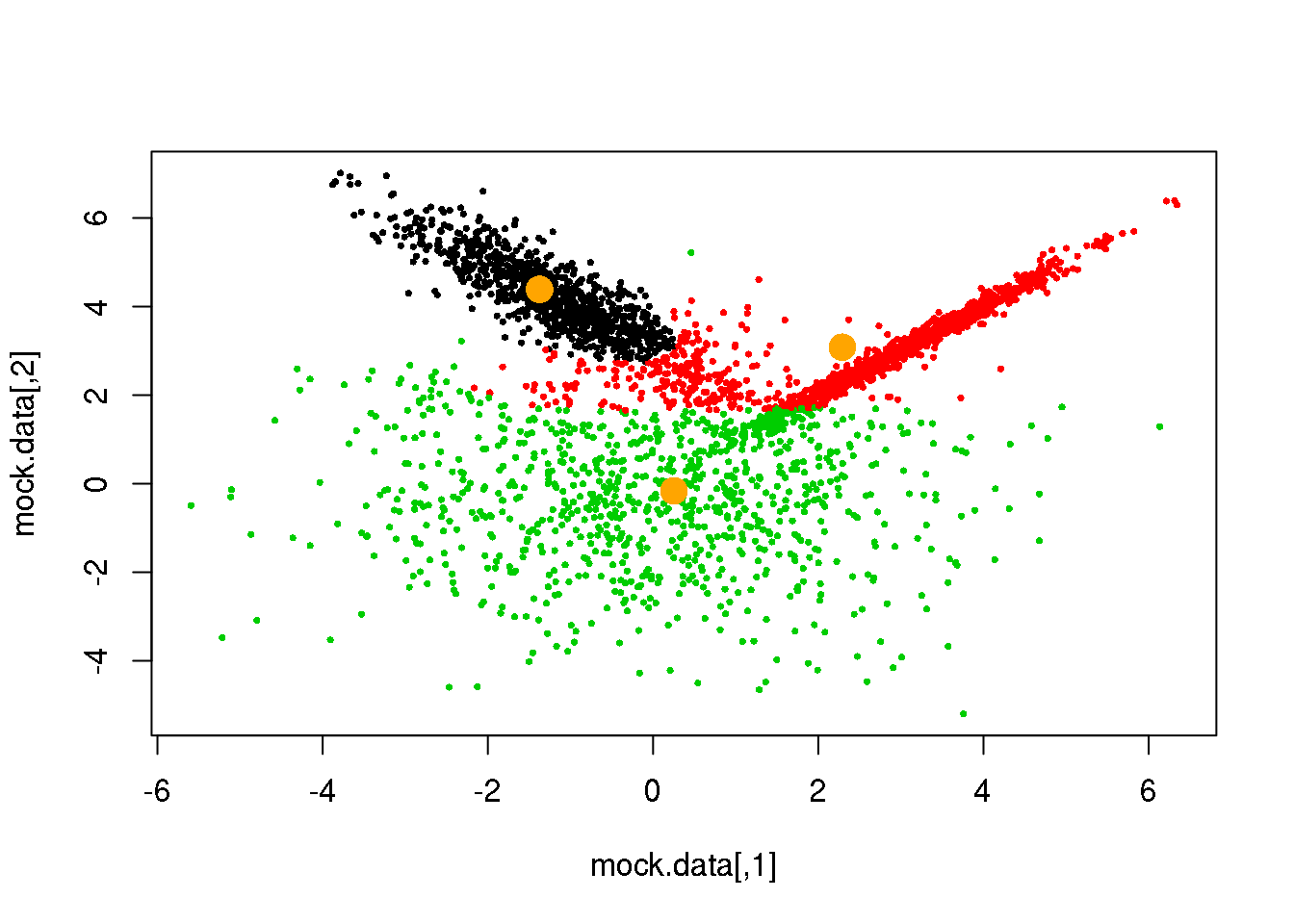
## [1] 173
## [1] 143
## [1] 89
## [1] 44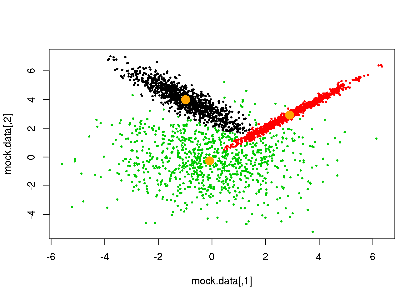
## [1] 8
## [1] 6
## [1] 0
Density based clustering
library("dbscan")
cluster <- dbscan(data[,-4],minPts = 5, eps=0.02)
mask <- cluster$cluster != 0
plot(data[,c(1,6)],pch=".")
points(data[mask,c(1,6)],pch=16,cex=.2,col=(cluster$cluster[mask]+1))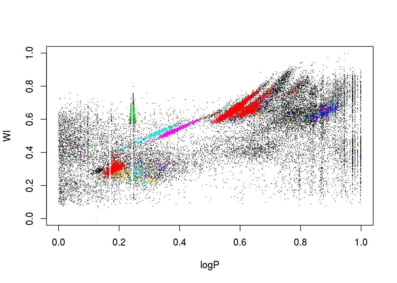
plot(data[,c(1,2)],pch=".")
points(data[mask,c(1,2)],pch=16,cex=.2,col=(cluster$cluster[mask]+1))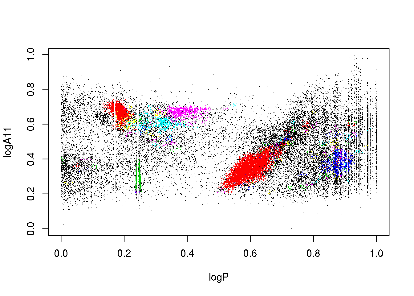
plot(data[,c(1,3)],pch=".")
points(data[mask,c(1,3)],pch=16,cex=.2,col=(cluster$cluster[mask]+1))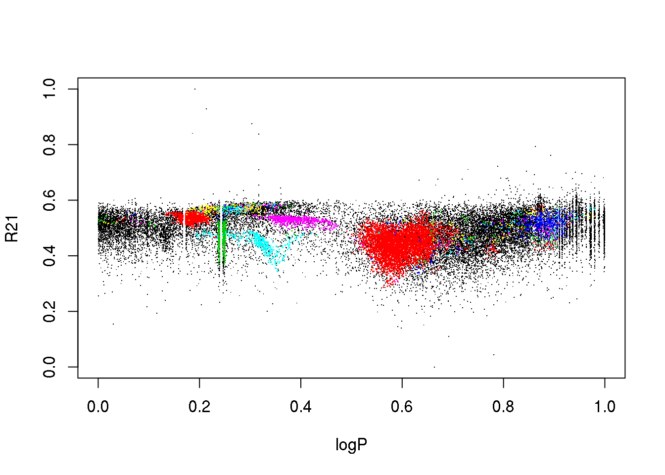
plot(data[,c(1,4)],pch=".")
points(data[mask,c(1,4)],pch=16,cex=.2,col=(cluster$cluster[mask]+1))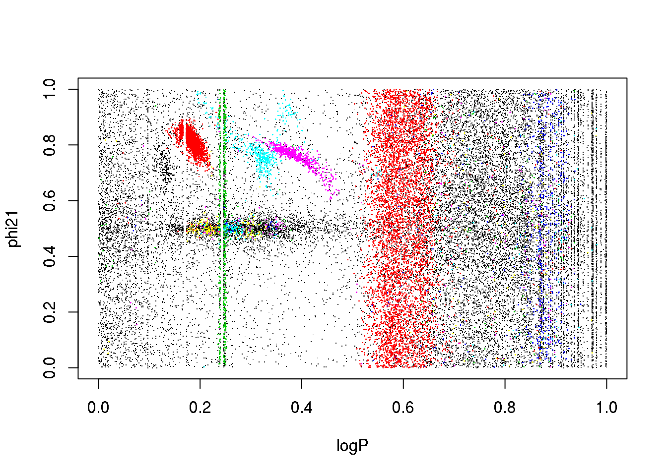
plot(data[,c(1,5)],pch=".")
points(data[mask,c(1,5)],pch=16,cex=.2,col=(cluster$cluster[mask]+1))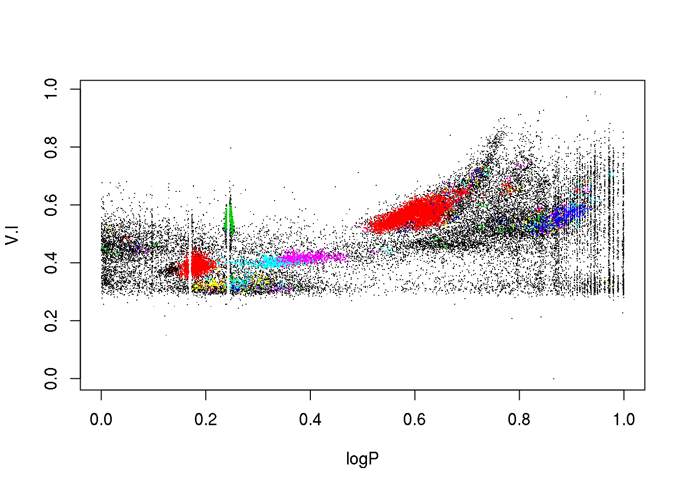
cluster <- optics(data[,-4],minPts = 15, eps=0.02)
res <- optics_cut(cluster, eps_cl = 0.0195)
mask <- res$cluster != 0
column <- 6
plot(data[,c(1,column)],pch=".")
points(data[mask,c(1,column)],pch=16,cex=.5,col=res$cluster[mask]+2)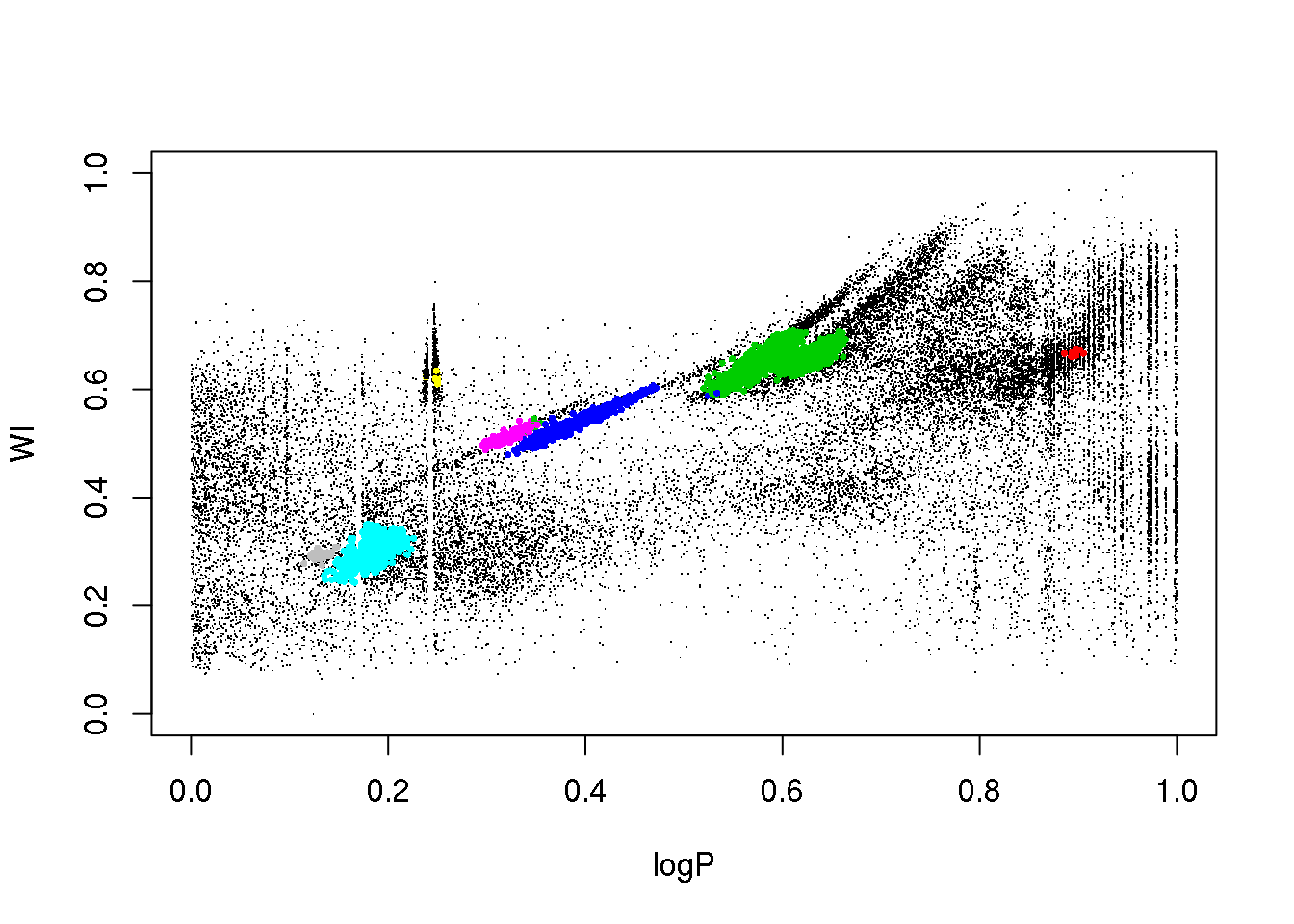
plot(data[,c(1,2)],pch=".")
points(data[mask,c(1,2)],pch=16,cex=.2,col=(cluster$cluster[mask]+1))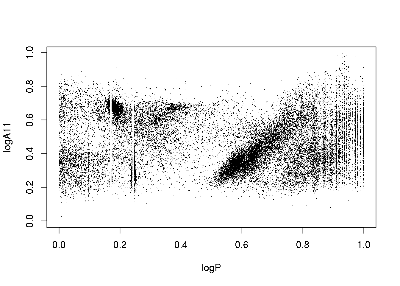
plot(data[,c(1,3)],pch=".")
points(data[mask,c(1,3)],pch=16,cex=.2,col=(cluster$cluster[mask]+1))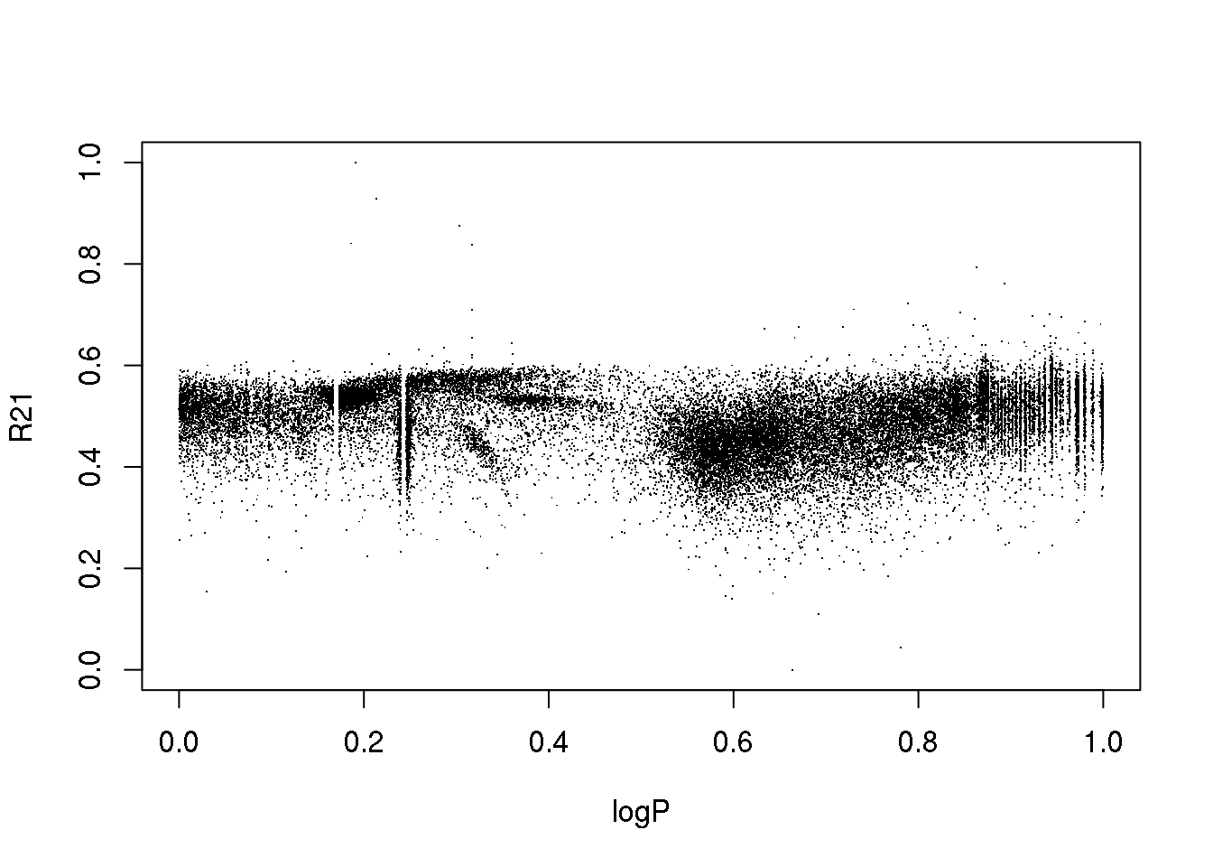
plot(data[,c(1,4)],pch=".")
points(data[mask,c(1,4)],pch=16,cex=.2,col=(cluster$cluster[mask]+1))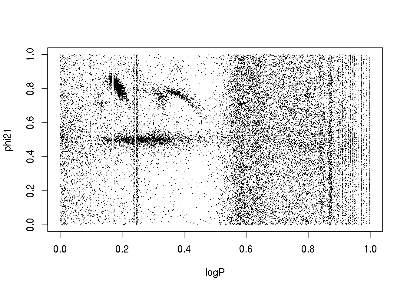
plot(data[,c(1,5)],pch=".")
points(data[mask,c(1,5)],pch=16,cex=.2,col=(cluster$cluster[mask]+1))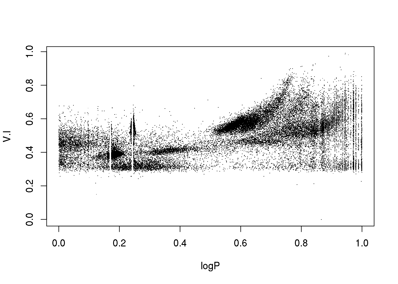
apply(data,2,range)## logP logA11 R21 phi21 V.I WI
## [1,] 0 0.0000000 0 2.429557e-05 0.0000000 0
## [2,] 1 0.9941714 1 9.999900e-01 0.9907912 1When I had to deal with this dataset, I actually used a different algorithm known a Hierarchical Mode Association Clustering (HMAC).
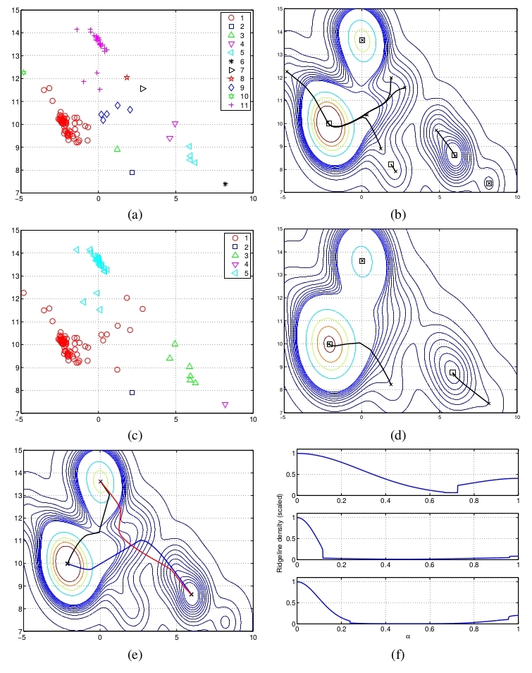
Kohonen
plot(mock.data)
library("kohonen")
## Loading required package: class## Loading required package: MASSlibrary("fields")## Loading required package: spam## Loading required package: grid## Spam version 1.0-1 (2014-09-09) is loaded.
## Type 'help( Spam)' or 'demo( spam)' for a short introduction
## and overview of this package.
## Help for individual functions is also obtained by adding the
## suffix '.spam' to the function name, e.g. 'help( chol.spam)'.##
## Attaching package: 'spam'## The following objects are masked from 'package:base':
##
## backsolve, forwardsolve## Loading required package: maps##
## Attaching package: 'maps'## The following object is masked from 'package:kohonen':
##
## map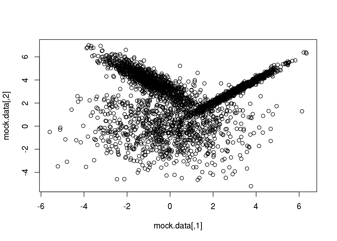
cluster <- som(mock.data)
plot(cluster, type="code")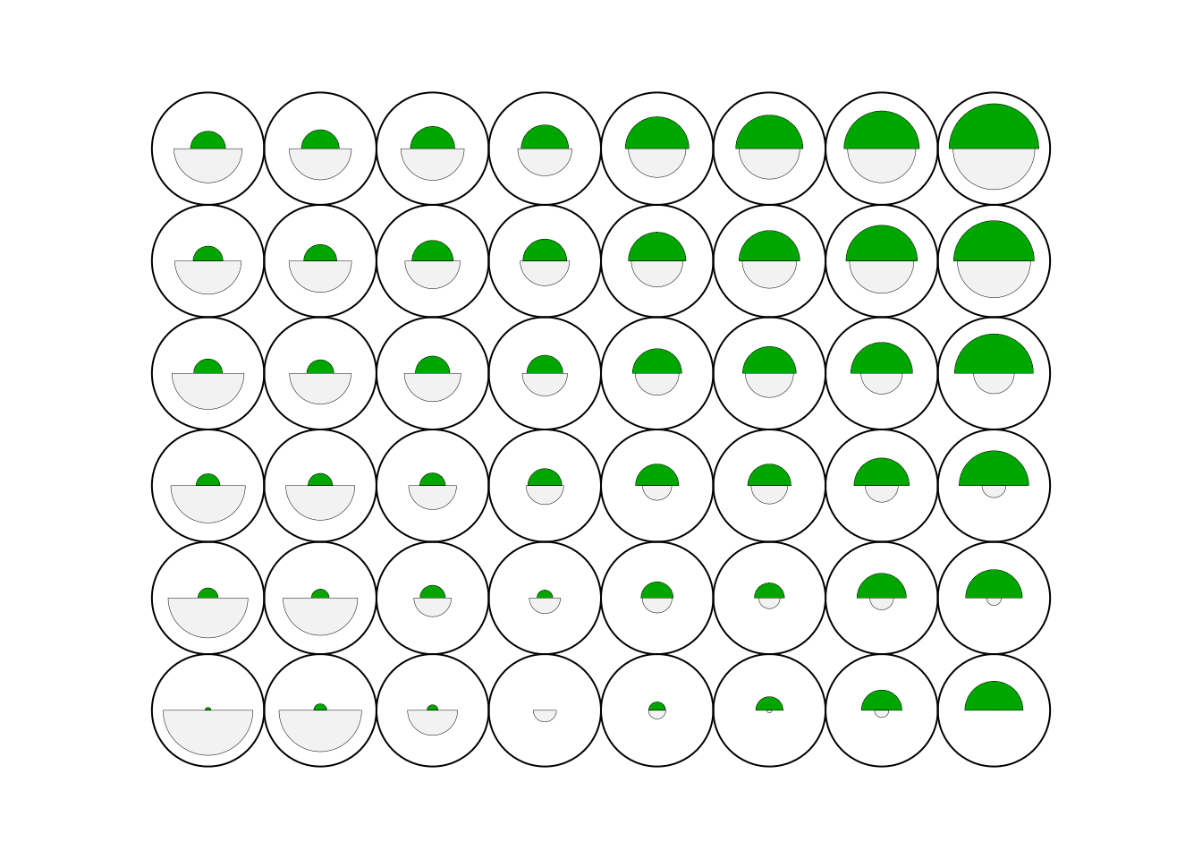
plot(cluster, type="changes")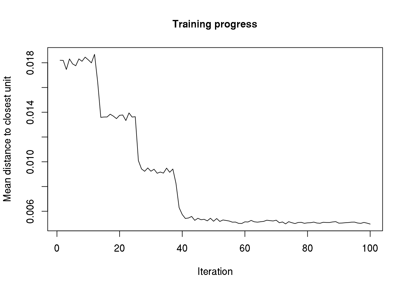
plot(cluster, type = "property", property = cluster$codes[,2], main=names(cluster$data)[2], palette.name=tim.colors)
plot(cluster, type="dist.neighbours")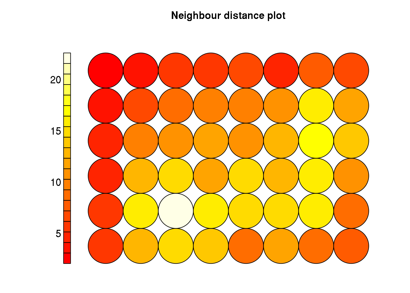
plot(cluster, type="count")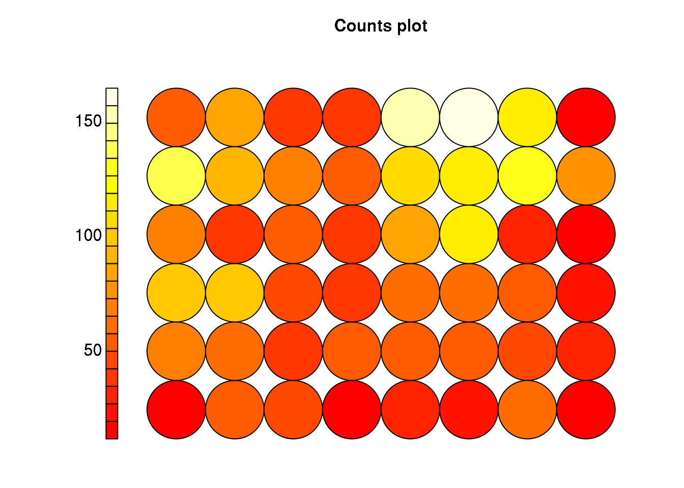
Hierarchical (connectivity based) clustering
##dists <- dist(data)
##clusters <- hclust(dists, method = 'average')
#clusters <- hclust(dists, method = 'ward.D')
#clusters <- hclust(dists, method = 'ward.D2')
#clusters <- hclust(dists, method = 'single')
#clusters <- hclust(dists, method = 'complete')
#clusters <- hclust(dists, method = 'centroid')
#clusters <- hclust(dists, method = 'median')
#clusters <- hclust(dists, method = 'mcquitty')
##plot(clusters)
##clusterCut <- cutree(clusters, 15)
##plot(data[,1],data[,6], col=clusterCut,pch=16,cex=.3)
##clusterCut <- cutree(clusters, 200)
##plot(data[,1],data[,4], col=clusterCut,pch=16,cex=.3)

##dists <- dist(data[,-4])
##clusters <- hclust(dists, method = 'average')
##clusterCut <- cutree(clusters, 200)
##plot(data[,1],data[,4], col=clusterCut,pch=16,cex=.3)

##dists <- dist(data[,-4])
##clusters <- hclust(dists, method = 'single')
##clusterCut <- cutree(clusters, 200)
##plot(data[,1],data[,4], col=clusterCut,pch=16,cex=.3)
Subspace clustering
Subspace clustering starts from the hypothesis that, although the data set has been drawn from a multi-variate distribution in D dimensions (usually \(\mathbb{R}^D\)), each cluster lives in a linear or affine subspace of the original space. Imagine for example, a data set in 3D, where the data points lie in 1. two planes for clusters 1 & 2 2. a line for cluster 3
The data set is the union of sets from each of the subspaces. The objective then is to find at the same time the cluster assignments, and the subspace definitions.
In mathematical terms, each subspace is defined as
\[ S_i = {x \in \mathbb{R}^D: x=\mathbb{\mu}_i+U_i\cdot\mathbb{y}} \]
where \(U_i\) is a matrix with the subspace basis vectors as columns, \(\mathbb{y}\) are the new coordinates in that basis, and \(\mathbb{\mu}_i\) is the centre (in the case of affine subspaces). Our goal is to find the \(\mathbb{\mu}_i\), \(U_i\), the dimensionality \(d_i\) of each subspace, and the cluster labels.
This can be achieved in a number of ways (see http://citeseerx.ist.psu.edu/viewdoc/summary?doi=10.1.1.225.2898 for a comprehensive, yet not particularly clear introduction):
Algebraic methods
Generative methods
Spectral methods
Here I will only explain the iterative version which is the simplest, although some of the features are shared amongst the various methods.
In the iterative approach, we start from a (possibly random) initial clustering (like, for example, \(k\)-means). Then, we alternate to steps consisting of:
- Calculating the Principal Components for each cluster and projecting the entire data set onto the first \(d_i\) components.
- Reassigning the points to the clusters that minimizes the reconstruction error, where the reconstruction error is defined as
\[ ||\mathbb{x}_j-(\mathbb{\mu}_i-U_i\cdot\mathbb{y}_j)|| \]
Problems: * the subspaces are linear
we have to have an initial clustering
We need to fix a priori the number of clusters and the dimensionality of the subspaces
#library("orclus")
#cluster <- orclus(data,k=10,l=3,180,inner.loops=20)
#plot(data[,1],data[,6],col=cluster$cluster,pch=".")
#for(i in 1:length(cluster$size)) {
#plot(as.matrix(data) %*% cluster$subspaces[[i]], col = cluster$cluster, ylab #= paste("Identified subspace for cluster",i))
#}

#for(i in 1:length(cluster$size)) {
#mask <- cluster$cluster==i
#plot(data[,1],data[,6],col="black",pch=".")
#points(data[mask,1],data[mask,6],col="red",pch=16,cex=.5)
#}
Spectral clustering
Spectral clustering can be better understood if we view the data set as an undirected graph. In the graph, data points are vertices that are connected by links with strength or weight. The weight is supposed to reflect the similarity between two vertices (points).
In principle, the graph can be constructed including links between all pairs of points, although this may be too computer intensive (imagine the case of Gaia wih \(10^9\) points: we would need \(10^18\) links). If we need to simplify the affinity matrix, we can include only links to points within an \(\epsilon\)-hyperball, or only to the \(k\)-nearest neighbours (this needs to be made symmetric).
Once we have the vertices and links/arcs, there are several ways to decide how we measure affinity or similarity (the weights). In the \(\epsilon\)-neighbourhood, there is no strong need to define a weight (they could all be set to one). But in the fully connected graph, we need a measure of affinity that has to be positive and symmetric for all pairs of points \(\mathbb{x}_i\) and \(\mathbb{x}_j\). The most popular by far is the Gaussian kernel:
\[s_{ij}=s(\mathbb{x}_i,\mathbb{x}_j) = K(\mathbb{x}_i,\mathbb{x}_j) = \exp(\frac{-||\mathbb{x}_i-\mathbb{x}_j||^2}{2\sigma^2})\]
Let \(S={s_{ij}}\) be the matrix of similarity (or adjancency) of the graph.
Now it would be time to look back at the kernel trick explanation yesterday. There are other choices of kernel to measure similarity.
So, in summary we are left with a graph which we want to partition. We would like to divide the graph into disjoint sets of vertices such that vertices within one partition have strong links, while at the same time links that cross cluster frontiers have weak weights. How do we do this? The answer has to do with Laplace…
One obvious (and potentially wrong) way to partition the graph is to find the cluster assignments that minimize
\[ \mathcal{W}=\sum_{i=1}^{k} S(C_i,\neg{C_i})=\sum_{k\in C,k\in \neg{C_i}} s(j,k) \]
where C and C’ are two clusters in our partition. It is potentially wrong because in many scenarios, the optimal solution would be to separate a single point. Hence, we need to bias the minimization process to avoid singular clusters. We could minimize \(\mathcal{W}\) divided (scaled) by the cluster size (which we can approximate by 1. the number of vertices or 2. the so-called partition volume).
- It turns out (but I will not prove it; it involves the Rayleigh-Ritz theorem) that minimizing (the scaled versions of) \(\mathcal{W}\) under some relaxation of the conditions is equivalent to finding the eigenvectors of the so-called Laplace matrix. Depending on the scaling of , the Laplace matrix can be normalized or unnormalized (but this is just jargon):
- \(L = D - S\), the unnormalized Laplace matrix (scaling by the number of vertices)
- Normalized Laplace matrices:
- \(L_{sym}=D^{-1/2}LD{^{-1/2}}\)
- \(L_{rw} = D^{-1}L\)
where \(D\) is the diagonal matrix formed by
\[d_{i}=\sum_{j=1}^{n}s(i,j) \]
- Now, once we have the graph fully specified, spectral clustering proceeds by computing the eigenvectors/eigenvalues of the Laplacian, and aplying \(k\)-means to the rows of the \(U\) matrix.
Spectral clustering with the unnormalized Laplacian

Excerpt from the tutorial by Ulrike von Luxburg
The (justified) hope is that the new space of characteristics is more separable than the original one. The new space of characteristics is
Spectral clustering with the normalized symmetric Laplacian
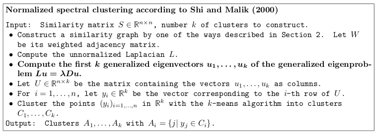
Excerpt from the tutorial by Ulrike von Luxburg
Spectral clustering with the normalized random walk Laplacian
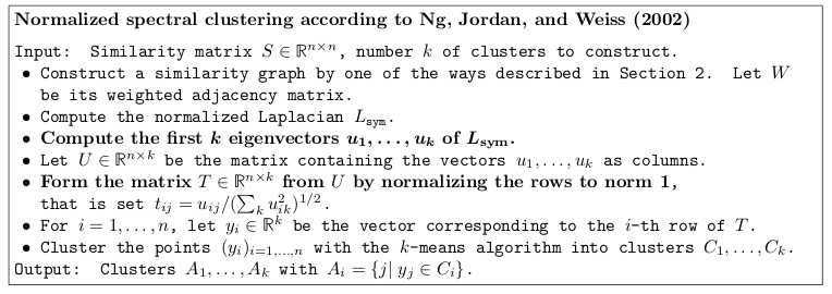
Excerpt from the tutorial by Ulrike von Luxburg
#library(kernlab)
#cluster <- specc(data,centers=25,kernel="rbfdot",kpar="automatic",
#                 nystrom.red=FALSE,nystrom.sample=5000,iterations=200)
Clustering evaluation measures
Connectedness
![Excerpt from the R clValid [package description] (ftp://cran.r-project.org/pub/R/web/packages/clValid/vignettes/clValid.pdf)](images/connectedness.jpg)
Excerpt from the R clValid [package description] (ftp://cran.r-project.org/pub/R/web/packages/clValid/vignettes/clValid.pdf)
Silhouette width

![Excerpt from the R clValid [package description] (ftp://cran.r-project.org/pub/R/web/packages/clValid/vignettes/clValid.pdf)](images/silhouette2.jpg)
Excerpt from the R clValid [package description] (ftp://cran.r-project.org/pub/R/web/packages/clValid/vignettes/clValid.pdf)
Dunn index
![Excerpt from the R clValid [package description] (ftp://cran.r-project.org/pub/R/web/packages/clValid/vignettes/clValid.pdf)](images/dunn.jpg)
Excerpt from the R clValid [package description] (ftp://cran.r-project.org/pub/R/web/packages/clValid/vignettes/clValid.pdf)
